 |
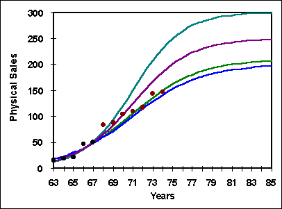
Figure 1, Fitting the logistics curve with sparse data |
| Forecasting sales or technology substitution during the early stages of new product introduction is extremely difficult but critical. The General Sales Growth CurvesSM is an simple, effective penetration model applicable to the growth phase of new products and technologies. In this paper, a two parameter model is shown to be effective for forecasting sales of expendable products when as few as 5 annual data points are available. This model has been tested effectively on over 300 product and technologies. |
1. Introduction
Sales and technology substitution forecasts using sparse data have always been
problematic. Penetration models have become increasingly complex in attempts to describe
the total product life cycle, include a range of influences, and improve precision [2, 3,
4, 9, 12, 13, 14]. Unfortunately, with only a few data points, such models are not usable.
The simplest models typically used for forecasting are the exponential curve (which is a
two parameter model representing constant proportional growth) and the simple logistics
curve (which is a three parameter symmetric "S" shape growth model).
Unfortunately, even three parameter models, like the logistics curve are too complicated
for use with sparse data. Martino [10] has shown that small errors in the estimation of
the ultimate maturation level that is required for, the three parameter logistics curve,
can have large effects on earlier time period forecasts.
In this paper we will propose the use of a specific two parameter growth model, the General Sales Growth CurveSM (GSGCSM) for early forecasts. This curve represents a declining proportional growth and, like the exponential model, is applicable only to the growth phase of product and technology life cycles.
In figure 1 is a set of logistics curves yielding the same degree of fit to 5 data points. The quality of fit improves only using data further along the trajectory, usually beyond the inflection point. This is the estimation problem discussed by Martino [10].
 |
Figure 1, Fitting the logistics curve with sparse data |
With sparse data, only a few parameters can be estimated. Under these circumstances the exponential growth curve is usually preferred [11] and will be used as a standard of comparison to the General Sales Growth Curve.
2. General Sales Growth Curve
Analysis of proprietary and published data over the past 15 years has suggested that the
dynamic behavior of expendable products have very similar characteristics during their
initial growth phase [1, 5]. Expendable products are considered to be consumed upon
purchase. They represent the application of a technology. Capital goods, such as
equipment, represents the technological capability. Sales of these products can be
considered to the equivalent of the integral of the General Sales Growth Curve and
is modeled as such. Physical sales of new products tend to grow extremely rapidly. This
high growth rate tends to decrease over time until, at some point, product sales mature
and level out. Eventually, the product sales will decline as newer products and
technologies replace older ones.
In testing of hundreds of cases, we have found that the shape of the sales curve for manufactured expendable products, during the growth phase, appears to be the same [9]. Initial academic research work in this area was sponsored by the Institute for the Study of Business Markets, Pennsylvania State University. The growth phase does not include the eventual plateau of sales. A relatively simple two parameter expression can describe this growth. It must be re-emphasized that this relationship only applies to the growth phase of the life cycle. The use of a growth curve, such as the General Sales Growth Curve or the Exponential assumes that the long term growth characteristics will continue into the future. Maturation is implicitly assumed to be caused by outside factors which does not influence growth.
For the purposes of forecasting, we generally take the General Sales Growth Curve to be an empirical finding. However, the stability of a universal function describing the process implies stable mechanisms. Several mathematical expressions can used to describe the stable sales growth trajectory that we refer to as the General Sales Growth Curve [7]. We have found that a modified Gompertz, however, describes the data well and facilitates curve fitting and forecasting [5, 6]. The general form is:
U = Po(1+i){t-to}(Uo/Po)R{t-to}
Note: Exponents may not be correctly shown in Mosaic, the form is U=(Po(1+i)^{t-to})*(Uo/Po[^R^{t-to}])
where U is the physical sales; i is the long term growth rate and R is a universal parameter. Po is the market potential in the year of commercialization, to. Uo is the physical sales volume in that year. This relationship can be rearranged, resulting in a two parameter model for curve fitting.
Ln{U}-t Ln{1+i} = A +B R
This form of the GSGC can be fit to data using linear regression. R and i are considered universal constants, 0.77 and 8% respectively. Figure 2 shows the typical fit of data to the GSGC. The potential line is derived from the curve fit data and represents an extension of the asymptotic limit of growth.
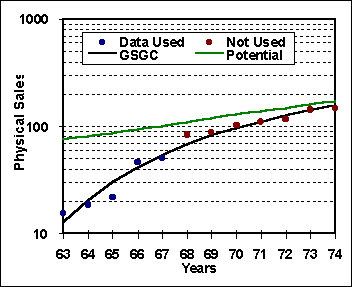 |
Figure 2, Typical fit of data to the General Sales Growth Curve |
3. Fitting Sparse Data
The GSGC has been found to be a surprising good sales forecasting tools with
proprietary sales data. That data usually contain several earlier years than are typically
available in public and commercial that are used in academic research. In those cases, a
few early data points have been found capable of describing a relatively long growth
period. This is particularly the case in materials and basic technologies. In figure 3 are
three cases from public data (Low Density Polyethylene Resin, Corn Exports, and Epoxy
Resins) where the GSGC is used to successful forecast 20 years of growth.
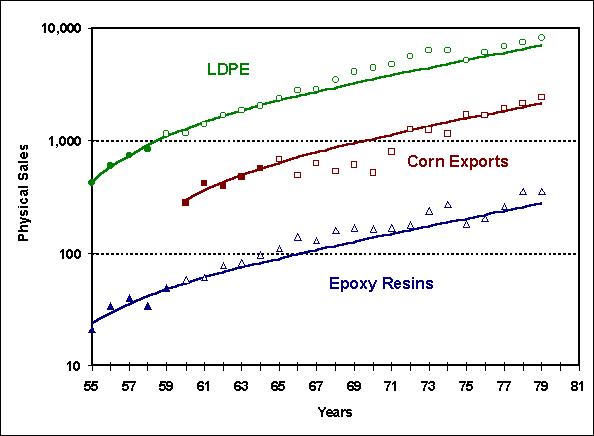 |
Figure 3, Typical Long Term Forecasts using the GSGC |
These examples are fairly typical of material business where the planning and development time frame is in the order of decades. Consumer products, however, tend to mature much more rapidly and therefore, a forecast restricted to the growth phase may not be appropriate.
4. Testing the Curves
Agreement of fit with historical data is a necessary condition for forecasting tools. The GSGC
was tested against the exponential model with 302 sets of manufactured products. This data
is from the Chemical Economic Handbook (SRI) and from the Historical Statistics of the
United States. Only early data, where growth exceeded 8% annually was used in the testing.
This data is independent of that originally used to determine the universal GSGC
parameters (R and i). Only segments of the data showing a significant
sustained annual growth greater were used. This assured that the data were limited to the
growth phase of the life cycle. The standard R-Squared was used as the measure of
"goodness of fit". It should be noted that because of the nature of growth, any
upward sloping curve, even a straight line, captures a major portion of the variation. On
average approximately 90% of the variance was captured by the General Sales Growth Curve
compared with only 77% with the simple exponential.
Below are listed test results by category of industry and geographic area. As can be seen, the GSGC out-performed the exponential in all industries and all but one geographic area. In some cases the difference between the GSGC and the exponential is striking for example in the case of the Farm Practices which showed a 32% improvement in the R-Squared.
Relative Fit (R-Squared, %)
| Industries | GSGC | Exponential | Difference |
| Pharmaceuticals | 85 | 80 | 5 |
| Farm Products | 90 | 71 | 19 |
| Consumer Products | 87 | 65 | 22 |
| Farm Practices | 96 | 64 | 32 |
| Wood Products | 90 | 80 | 10 |
| Petroleum/Energy | 90 | 76 | 14 |
| Polymers | 90 | 76 | 14 |
| Technologies | 92 | 72 | 20 |
| Chemicals | 92 | 68 | 24 |
| Applications | 90 | 82 | 8 |
| Geographic Areas | |||
| Western Europe | 93 | 85 | 8 |
| Japan | 81 | 82 | -1 |
| Soviet Block | 93 | 92 | 1 |
| Developing Countries | 93 | 86 | 7 |
It should be noted that there is a broad range of performance using the GSGC. Many of the cases showed extra ordinary good fit of data covering long time ranges.
GSGC, R-Squared (%)
| Industries | Max. | Min. |
| Pharmaceuticals | 99 | 65 |
| Farm Products | 96 | 67 |
| Consumer Products | 96 | 63 |
| Farm Practices | 99 | 91 |
| Wood Products | 96 | 83 |
| Petroleum/Energy | 99.6 | 87 |
| Polymers | 99.5 | 70 |
| Technologies | 99 | 72 |
| Chemicals | 98 | 71 |
| Applications | 99 | 68 |
| Geographic Areas | ||
| Western Europe | 99.6 | 81 |
| Japan | 97 | 61 |
| Soviet Block | 99.7 | 82 |
| Developing Countries | 99.7 | 84 |
5. Testing Forecasts
However, merely describing data well is insufficient for a model to be effective as a forecasting tool. The model has produced reliable forecasts. To test these models we selected a subset of 148 data sets for which there were at least 10 years of growth data. Growth exceeding 95% over the first five years of data available without any missing data. The length of the time frame was selected to give a sufficiently large sample and still have enough data points to permit the testing of the forecast. The number of cases, publicly available, with growth data of 20 years or greater was insufficient for reliable testing. Five data points were used to construct the forecasts and following five years were used to test the results. The results are shown on Figures 4 through 8.
The most catastrophic problem in forecasting is being way off. Figure 5 shows the percentage of forecasts that predicted volume over 100% greater than actual for the two models. It should be noted that the exponential or constant percentage growth model is notorious for giving highly optimistic forecasts for new products. Over 60% of the exponential model forecasts for the fifth year were off by more than 100% compared to approximately 15% using the GSGC. During the second year, approximately 5% of the GSGC forecasts were greater than 100% in error while over 30% of the exponential forecasts were over this limit.
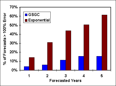 |
Figure 4, Fraction of forecasts with over 100% deviation from actual |
The difference between these models is even more striking when considering the average error. Figure 5 shows the average deviation. In order to cover the full range, a logarithm scale had to be used. On average, the GSGC showed a 10% error in the first year compared to a 40% for the exponential. The error for both models grows as the forecast is extended. However, the average error for the GSGC seems to level out at 45% while that of the exponential continues to accelerate reaching over 4000% by the fifth year.
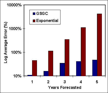 |
Figure 5, Average Deviation from Actual |
Figure 6 shows the average absolute deviations. The average absolute deviation captures the total variability between forecast and actual. For both the GSGC and the exponential curves this measure is inherently larger than the simple average deviation. However, the same trend is clear, the GSGC gives a fair better forecast.
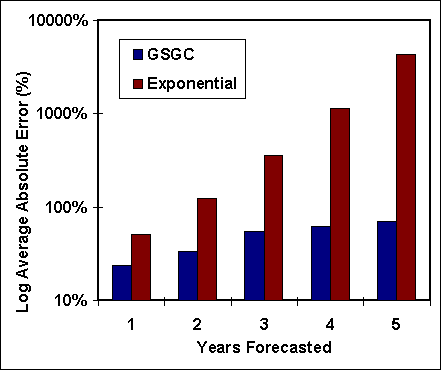 |
Figure 6, Average Absolute Deviation from Actual |
Figures 7 and 8 show the distributions of forecast errors for the first and fifth years respectively. The deviations of the GSGC are far more concentrated than that of the exponential.
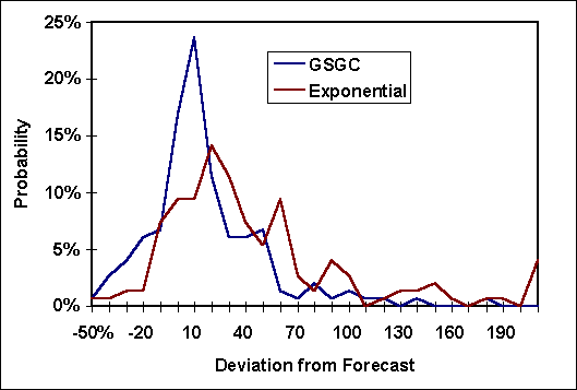 |
Figure 7, Deviation of first year forecast from actual |
The deviation distribution is skewed to the right as one would expect given a natural lower limit of negative one hundred percent and no upper limit to the deviation. For the fifth year the upper distribution tail dominates the exponential forecast while the forecasts from the GSGC are still concentrated toward the lower part of the error distribution.
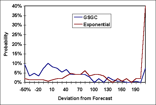 |
Figure 8, Deviation of fifth year forecast from actual |
Total industry data was used in these tests. Such data is less tightly controlled than proprietary sales information available within firms. Analysis of proprietary data has indicated that even greater predictability can be realized. Removing uncertain data points and can, furthermore, greatly improve forecasts.
6. Implications and Directions for Future Research
It should be noted that the data sets used for testing span over 200 years. Some of the series ran as much 175 years. These included, for example, cotton from the advent of the cotton gin and the registration of steam boats from the first decade of the 19th century. While the majority of the data were recent, the analysis does imply some degree of gross time independence. If the GSGC is truly general and represents a universal principle, then it could be the basis of general product and technology diffusion modeling process.
It should be noted, however, that the General Sales Growth Curve implies invariance of the rate of penetration. If GSGC is universal, dynamics of penetration, though not the potential into which a product or technology is growing, is independent of its characteristics, its value, time, or the method of delivery. These factors do influence, whether the growth will continue or even would start. The GSGC model essentially says that if dynamic growth exists, it follows a given trajectory into a potential set by the characteristics of the product.
As has been shown, the General Sales Growth Curve is a fairly accurate forecasting tool. However, there is still systematic error in the forecasted results. The deviations are general on the positive side. This results in an almost consistent over-estimate of actual performance. In practice, this is not a major problem since GSGC estimates tend to be used for auditing forecasts obtained by other means. However, it leads one to expect that some improvement in the form of this curve is feasible.
References
1. Bass, F.M., "A New Product Growth Model for Consumer Durables", Management Science 15 (1969), pp. 215-227
2. Chaffrey, J. M., G. Lilien (1980) Market Planning for New Industrial Products, New York, John Wiley
3. Horskey, D. "A Diffusion Model Incorporating Product Benefits, Price, Income and Information", Marketing Science, 9 (1990) pp. 342-365
4. Jain, D., Mahajan, V., Muller, E., " Innovation Diffusion in the Presence of Supply Restrictions", Marketing Science, 10 (1991) pp. 83-90
5. Jepson, C., E. I. DuPont de Nemours & Co., Inc, Internal Presentation (1976)
6. Lakhani, H., "Empirical Implications of Mathematical Functions Used to Analyze Market Penetration of New Products", Technological Forecasting and Social Change, 15 (1979)
7. Lee, J. C., Lu, K. W., "Algorthm and Practice of Forecasting Technological Substitution with Data Based Transformed Models", Technological Forecasting and Social Change, 36 (1980) pp. 401 - 414
8. Lieb, E. B., Gross, I, "A General Product Sales Growth Curve", International Meeting of TIMS, (1985)
9. Mahajan, V., Muller, E., Bass, F. M., "New Product Diffusion Models in Marketing: A Review and Directions for Research", Journal of Marketing, 54 (1990), pp 1-26
10. Martino, J. P., "The Effect of Errors in Estimating the Upper Limit of a Growth Curve", Technological Forecasting and Social Change, 4 (1972) pp. 77-84
11. Murray, S. O., Rankin, J. H., "Use Diffusion: An Extension & Critique", Technological Forecasting and Social Change, 16 (1980) pp. 331-341
12. Olson, J. A., "Generalized Least Squares & Maximum Likelihood Estimation of the Logistic Function for Technological Diffusion", Technological Forecasting and Social Change, 21 (1982) pp. 241-249
13. Oren, S. S., Rothkapt, M. H., "A Market Dynamic Model for New Industrial Products and Its Applications", Marketing Science, 3 (1984) pp. 247-265
14. Schmittlein D., Mahajan, V. "Maximum Likelihood Estimation for an Innovation Diffusion Model for New Product Acceptance", Marketing Science, 1 (1982) pp. 57-78